
Since I'm a space nerd, I decided to use the dataset of NASA astronauts recruited between 1959 and 2009 to make things more interesting. In this article, I'll outline the key steps and decisions taken during data preprocessing, and demonstrate machine learning methods that I applied to perform the analysis. My primary objective is to find correlations between astronauts' educational, military, and demographic backgrounds and whether or not those correlations have anything to do with the astronauts' consecutive number of spaceflights. My secondary objective is to attempt to build a model that could be used to predict the demographic, educational, and military background of the next astronauts (or the other way around? I'm not sure, let's find out). I also want to demonstrate some of the most interesting results.
Data Used
For this analysis, I used data that can be downloaded from https://www.kaggle.com/nasa/astronaut-yearbook. The dataset contains 357 observations of 18 variables in a CSV format. The dataset has several columns with empty or NA values, including some that need imputation, separation, and conversion to factors. I'm doing this because according to Wickham and Grolemund (2017), raw datasets are usually unsuitable for data visualisation "out of the box", therefore I need to transform the dataset, and for this purpose, I'm going to use tidyverse packages such as dplyr, tidyr, and stringr to select, filter, mutate, separate, and summarise the data.
There is a similar analysis of NASA astronauts conducted by Smith et al. (2020), where the authors analysed the change in astronauts' demographics over time using a regression modeling of a much larger dataset. Smith et al. also used the GLiM and GENLIN methods. However, in my analysis, I'm choosing variables such as astronauts' Age.at.Selection and the number of spaceflights to conduct a simpler linear regression proposed by Toomey (2014).
Machine Learning Methods Used
According to Toomey (2014), a Decision Tree algorithm can be applied to predict the target value based on the predictor variable. I'll use this algorithm to examine the number of spaceflights based on the astronauts' demographics, education, and military rank, labeled in the dataset as Age.at.Selection, First.Grad.Major, and Military.Rank. Another algorithm that I'm going to use will be a Random Forest, which according to Toomey (2014), can be utilised to create multiple decision trees, and will allow me to select the best as a final result. James et al. (2021) argued that Random Forests can be applied to datasets with a large number of predictor values. Therefore, I think this algorithm should be able to predict the number of spaceflights based on the choice of predictor (if that makes sense?).
Practical: Data Preprocessing
I'm using R studio, where I define a raw data variable and load the data from a CSV file using the read.csv() method. My initial observation is that the data contains values that could be separated into multiple columns. Doing so, for example, would enable me to identify the importance of the first undergraduate major and the likelihood of becoming an astronaut. Moreover, I was interested in seeing continuous variables such as the astronauts' age, in order to determine how candidates' changing age impacted their success in being selected during the astronaut selection process. To achieve this, I wrote a simple function called get_age() as shown below:
get_age = function (year1, year2) {
  # If year2 is not empty, then the astronaut is deceased
  # If year2 is not empty, then the astronaut is deceased
  if (is.na(year2) || year2 == '') {
    year2 = 2021
  }
  # Return age as a numeric value
  return (as.numeric(year2 - year1))
}
I modified the dataset further by adding new columns such as Age.at.Selection, First.Grad.Major, and Num.Grad.Major. Additionally, I removed astronauts who didn't reach the Kármán line of 100km above the mean sea level, officially known as "the edge of space" (Smith et al., 2020). Below is a code sample of a simple data wrangling with R:
# Assign transformed data into a new variable
data = rawdata %>%
  # Separate Birth.Date into Month, Day and Year
  separate(Birth.Date, sep = '/', into = c('Birth.Month', 'Birth.Day', ‘Birth.Year')) %>%
  # Omit some lines of code for brevity
  ...
  # Calculate the astronaut’s age using get_age custom function
  mutate(Age = get_age(Birth.Year, Death.Year), .after = 'Birth.Year') %>%
  ...
  # Transform characters into factors
  mutate_if(is.character, as.factor) %>%
  # remove astronauts who did not reach the The Kármán line of 100 km above mean sea level
  filter(Space.Flight..hr. > 0)
I also removed variables that I thought to be irrelevant to the analysis. Therefore, I removed 18 variables as shown below:
# Add column with a unique row identifier
data = tibble::rowid_to_column(data, ‘id')
# Remove unimportant data using “-c"
data = select(data, -c(Birth.Year, Birth.Month, Birth.Day, Birth.City, Death.Year, Death.Month, Death.Day,
Death.Mission, Status, Second.Alma.Mater, Third.Alma.Mater, Fourth.Alma.Mater, Fifth.Alma.Mater,
Sixth.Alma.Mater, Second.Undergrad.Major, Second.Grad.Major, Third.Grad.Major, Fourth.Grad.Major))
According to McGarry (2021), the dataset can be analysed with VIM and Hmisc packages to determine the variable with missing values, therefore as shown below, I utilised those packages to identify variables with missing values.
# Get sample of missing values
data.mis = prodNA(data, noNA = 0.1)
# Create visualization of missing values
aggr(data.mis, col = c('navy', 'yellow'), numbers = TRUE, sortVars = TRUE, labels = names(data.mis), cex.axis =
0.7, gap = 3, ylab = c('Missing Data', 'Pattern'))
# Impute missing values
data.impute = aregImpute(~Group+Year+Age+Age.at.Selection, data = data.mis, n.impute = 5)
The produced histogram and matrix revealed that the key variables, e.g., Group, Year, Age, and Age.at.Selection needed imputation. I used the MICE package for this purpose as shown in the code sample below:
# Use MICE package to impute missing values
impute_data = select(data, Group, Year, Age, Age.at.Selection)
mice_imputes = mice(impute_data, m = 5, maxit = 5)
mice_imputes$method
summary(mice_imputes)
# Test goodness of fit of imputed data
xyplot(mice_imputes, Group ~ Year | .imp, pch = 20, cex = 1.2)
densityplot(mice_imputes)
stripplot(mice_imputes, pch = 20, cex = 1.2)
Upon investigation of XY plots generated by the MICE package, I noticed that the goodness of fit of data is plausible, however, the density plot revealed that values imputed for the Group and Year variables don't match the dataset. To improve the goodness of fit, I removed Age.at.Selection and imputed this variable separately. This action provided better results, as shown in Figure 1 (right diagram).
 Figure 1: The comparison of density plots
Practical: R Programming Content
Functions
Wickham and Grolemund (2017) argued that functions are useful for automating repeated tasks. Therefore, I wrote a few custom functions to help me during the data analysis. The get_age() function proved to be useful for calculating astronauts' age. Another function test_cor() accepts two arguments and prints the output of t-tests and shows a correlation in the console log, including a simple XY plot:
# Run multiple correlation testing in one function
test_cor = function (var1, var2) {
  print(t.test(var1, var2))
  print(cor.test(var1, var2))
  pearson = cor(var1, var2, method = 'pearson')
  print('Pearson correlation: ')
  print(pearson)
  # Check the pearson correlation coefficient
  if (pearson < 0) {
    print('Correlation coefficient is negative!')
  } else if (pearson > 0 && pearson <= 0.1) (
    print('Correlation coefficient has small effect.')
  ) else if (pearson > 0.1 && pearson <= 0.5) {
    print('Correlation coefficient has medium effect.')
  } else if (pearson < 0.5) {
    print('Correlation coefficient has large effect!')
  }
  spearman = cor(var1, var2, method = 'spearman')
  print('Spearman correlation: ')
  print(spearman)
  plot(var1, var1)
}
# Example usage
test_cor(data$Space.Flights, data$Year) # Small
test_cor(data$Space.Flights, data$Space.Walks..hr.) # Medium
test_cor(data$Space.Flights, data$Space.Flights) # High
On the other hand, I wrote the showDistribution() function to visualise the distribution of a variable on the plot. I wrote a similar function showDistribution2() to plot two variables on the same plot.
# Visualising distribution
showDistribution = function (data, variable, plot = 'bar', xlabr = FALSE) {
  # Examine distribution of categorical variable using barchart
  if (plot == 'bar') {
    plot = ggplot(data) +
      geom_bar(mapping = aes(x = variable), fill = c('steelblue'))
    if (xlabr == TRUE) {
      plot = plot + scale_x_discrete(guide = guide_axis(angle = 90))
}
plot }
  # Overlay multiple histograms in the same plot using geom_freqpoly
  else if (plot == 'freqpoly') {
    ggplot(data, mapping = aes(x = variable)) +
      geom_freqpoly(binwidth = 0.1)
  }
  # Show histogram - clusters of similar values suggest subgroups
  else if (plot == 'histogram') {
    ggplot(data, mapping = aes(x = variable)) +
      geom_histogram(binwidth = 0.1)
  } else {
    print('Plot not found!')
} }
Data Modelling
I used the above function (_showDistribution) to show the correlation between two variables using the Pearson and Spearman methods. In order to build a simple linear regression model, I used two R's functions called plot and abline as shown in the code sample below:
# Create a data frame with First Undergrad Majors over Time
subject_over_time = select(data, First.Undergrad.Major, Year) %>%
  filter(First.Undergrad.Major == 'Mechanical Engineering') %>%
  group_by(Year) %>% count(First.Undergrad.Major) %>% arrange(Year) %>%
  transmute(Year = Year, Astronauts = n)
# Plot the timeline of undergraduate majors between 1959 and 2009
plot(subject_over_time, main = 'Undergraduates with Mechanical Eng. Major’)
# Add a fit line
abline(lm(subject_over_time$Astronauts~subject_over_time$Year), col = 'red')
Machine Learning
After data preprocessing and modeling, it was time to try machine learning. As shown in the code sample below, I decided to use a Decision Tree algorithm to determine the most important feature provided in the algorithm's formula:
# Age at Selection is important, Gender is not even considered
demographics = subset(data, select = c(Space.Flights, Age.at.Selection, Gender))
demographics_model = rpart(formula = Space.Flights ~ ., data = demographics)
summary(demographics_model)
fancyRpartPlot(model = demographics_model, main = "Space Flights by Age at Selection")
Then, I used a Random Forest. The algorithm takes the variables of interest to assess their importance on Space.Flights variable, as shown in the code sample below:
# Generate the model
fit = randomForest(formula = Space.Flights ~ Age.at.Selection + Num.Undergrad.Major + Num.Grad.Major +
Num.Alma.Mater + Gender + Military.Rank + Military.Branch, data = data, ntree = 500, keep.forest = TRUE,
importance = TRUE, type = 'unsupervised')
# Age.at.Selection has significant importance on number of space flights, followed by the military rank and the
number of universities attended by each astronaut
importance(fit)
Practical: Display of Data and Results
Demographics
My analysis shows that contrary to the female astronauts, the number of male astronauts steadily increases over time (see Figure 2).
 Figure 2: The number of male vs female astronauts over time
However, there seems to be equal distribution of astronauts based on their age during the selection process. As shown in Figure 3, the mean age is 34.5. Interestingly, when compared between male and female astronauts, it turns out that female astronauts tend to be younger by 2 years.
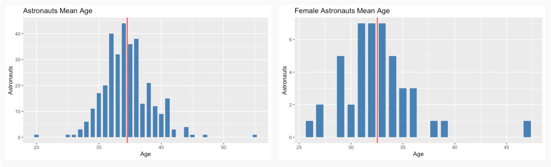 Figure 3: The mean age of astronauts (overall, male, female)
Education
The data shows that NASA favoured graduates from STEM courses. Although physicists are at the top of the list, individuals who studied engineering were more likely to become astronauts. Moreover, there is a trend showing a rise in undergraduates with mechanical engineering majors, as shown in Figure 4.
 Figure 4: Top 5 subjects studied at university
Military
The data shows that there are 195 astronauts with a military background which stands for 59.1%. When compared with the data shown in Figure 5 (left diagram), I was unsurprised to see that most of the number of astronauts who served in the US Navy steadily increased over time, in comparison to US Air Force, where the trend is slightly downwards.
 Figure 5: Astronauts serving in US Navy and US Air Force between 1959 and 2009
Other Results
The results of a Decision Tree algorithm shows that Age.at.Selection has the highest impact on the number of spaceflights. As shown in Figure 16, NASA is likely to select astronauts over 32 years of age for their spaceflights, and those astronauts can expect to go to space at least 3 times.
Code Listing
If you want to access the full source code, please send your request to chris.prusakiewicz@gmail.com. I'll be happy to send you a copy of the R file.
Conclusions
In summary, I find it difficult to arrive at any conclusion with regard to whether or not a demographic, educational, or military background has any significant role in the astronauts' number of spaceflights. The data analysis shows that results are limited to only a few factors, e.g., Age.at.Selection and Military.Rank. However, these shouldn't be considered as predictor values, because this analysis has several limitations. Firstly, astronauts' sex doesn't seem to have any influence, despite the fact that the majority of them are male. Secondly, astronauts' education doesn't seem to provide any insight into whether or not it increases the chances of going to space. Therefore, future work should consider better techniques of data transformation, perhaps changing categorical variables such as Alma.Mater, Undergraduate.Major, and Graduate.Major into numerical values could potentially improve models and algorithms implemented in this analysis. Removal of outliers, i.e., astronauts with a higher number of spaceflights than usual, and a logarithmic transformation could be applied to create more linear patterns (Wickham and Grolemund, 2017).
Refereces
James, G., Witten, D., Hastie, T. and Tibshirani, R. 2021. An Introduction to Statistical Learning with Applications in R. Springer, 2nd edn.
kaggle.com (2021) NASA Astronauts, 1959 to present [Online] Available at: https:// www.kaggle.com/nasa/astronaut-yearbook [Accessed: 11 November 2021].
McGarry, K. (2021) 6.3: Activity RStudio - Data Imputation for missing values [Online] Available at: https://study.online.sunderland.ac.uk/courses/278/pages/6-dot-3-activity-rstudio-data- imputation-for-missing-values?module_item_id=18420 [Accessed: 12 November 2021].
Smith, G.M., Kelley, M. and Basner, M. 2020. A brief history of spaceflight from 1961 to 2020: An analysis of missions and astronaut demographics. Acta Astronautica, Volume 175, p. 290-299, doi: https://doi.org/10.1016/j.actaastro.2020.06.004 Toomey, D., 2014. R for data science. Packt Publishing Ltd.
Wickham, H. and Grolemund, G., 2017. R for Data Science. Import, Tidy, Transform, Visualise and Model Data. O’Reilly Media, Inc.


